Day - 3 Preprocessing and Differential Expression

3.1 Learning Objectives

By the end of Day 3, you will be able to:

Apply different normalization methods to proteomic data
Perform batch effect correction
Conduct differential expression analysis using limma
Interpret and visualize differential expression results
Create volcano plots and MA plots

3.2 Module 1: Data Preprocessing

3.2.1 Why Normalize?

Normalization removes systematic technical variation to:

Make samples comparable
Reduce technical noise
Preserve biological signal

3.2.2 Loading Example Data

# Create example proteomic dataset with technical variation
set.seed(123)

n_proteins <- 500
n_samples <- 16

# Sample metadata
sample_metadata <- data.frame(
  sample_id = paste0("S", 1:n_samples),
  condition = rep(c("Control", "Treatment"), each = 8),
  batch = rep(c("Batch1", "Batch2"), times = 8),
  replicate = rep(1:8, times = 2),
  stringsAsFactors = FALSE
)

# Generate base protein abundances
protein_matrix_raw <- matrix(
  rnorm(n_proteins * n_samples, mean = 20, sd = 3),
  nrow = n_proteins,
  ncol = n_samples
)

rownames(protein_matrix_raw) <- paste0("P", sprintf("%05d", 1:n_proteins))
colnames(protein_matrix_raw) <- sample_metadata$sample_id

# Add biological effect (differential proteins)
de_proteins <- 1:50
protein_matrix_raw[de_proteins, sample_metadata$condition == "Treatment"] <- 
  protein_matrix_raw[de_proteins, sample_metadata$condition == "Treatment"] + 
  rnorm(50 * 8, mean = 2, sd = 0.5)

# Add batch effect
batch1_samples <- sample_metadata$batch == "Batch1"
protein_matrix_raw[, batch1_samples] <- protein_matrix_raw[, batch1_samples] + 1.5

# Add some missing values
missing_idx <- sample(1:length(protein_matrix_raw), size = 500)
protein_matrix_raw[missing_idx] <- NA

cat("Raw data dimensions:", dim(protein_matrix_raw), "\n")
#> Raw data dimensions: 500 16
cat("Missing values:", sum(is.na(protein_matrix_raw)), "\n")
#> Missing values: 500

3.2.3 Handling Missing Values

# Strategy 1: Remove proteins with too many missing values
threshold <- 0.3  # Remove if >30% missing
missing_per_protein <- rowSums(is.na(protein_matrix_raw)) / ncol(protein_matrix_raw)
filtered_proteins <- missing_per_protein <= threshold

protein_matrix_filtered <- protein_matrix_raw[filtered_proteins, ]

cat("Proteins after filtering:", nrow(protein_matrix_filtered), "\n")
#> Proteins after filtering: 499

# Strategy 2: Imputation (simple mean imputation)
protein_matrix_imputed <- protein_matrix_filtered

for (i in 1:nrow(protein_matrix_imputed)) {
  missing_idx <- is.na(protein_matrix_imputed[i, ])
  if (any(missing_idx)) {
    protein_matrix_imputed[i, missing_idx] <- mean(protein_matrix_imputed[i, ], na.rm = TRUE)
  }
}

cat("Missing values after imputation:", sum(is.na(protein_matrix_imputed)), "\n")
#> Missing values after imputation: 0

3.2.4 Normalization Methods

3.2.4.1 1. Median Normalization

# Calculate median for each sample
sample_medians <- apply(protein_matrix_imputed, 2, median, na.rm = TRUE)
global_median <- median(sample_medians)

# Normalize
protein_matrix_median <- protein_matrix_imputed
for (i in 1:ncol(protein_matrix_median)) {
  protein_matrix_median[, i] <- protein_matrix_median[, i] - 
    sample_medians[i] + global_median
}

# Visualize before and after
par(mfrow = c(1, 2))
boxplot(protein_matrix_imputed, main = "Before Median Normalization",
        las = 2, cex.axis = 0.7, ylab = "Abundance")
boxplot(protein_matrix_median, main = "After Median Normalization",
        las = 2, cex.axis = 0.7, ylab = "Abundance")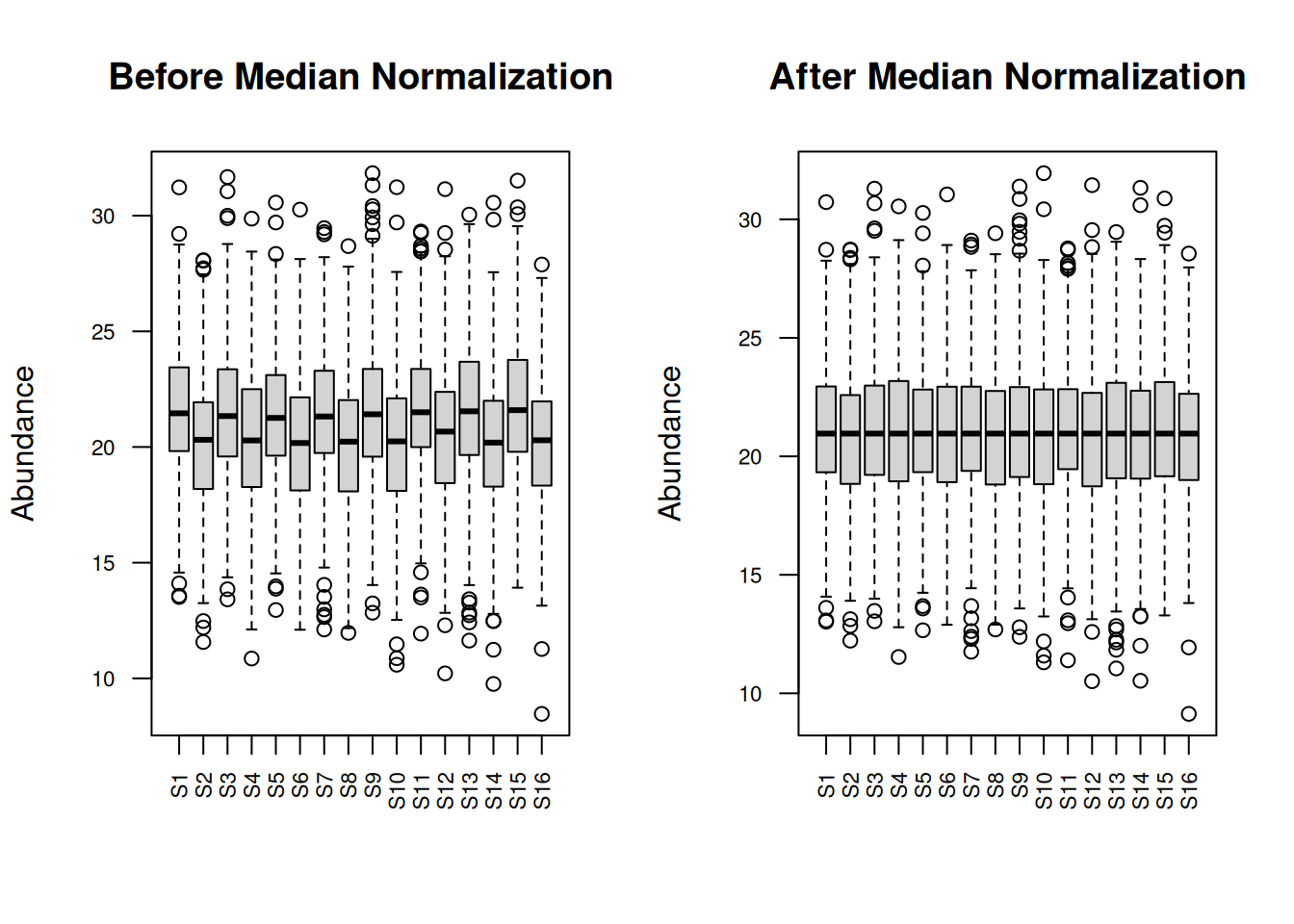

3.2.4.2 2. Quantile Normalization

# Quantile normalization
protein_matrix_quantile <- limma::normalizeBetweenArrays(protein_matrix_imputed, 
                                                          method = "quantile")

# Visualize
par(mfrow = c(1, 2))
boxplot(protein_matrix_imputed, main = "Before Quantile Normalization",
        las = 2, cex.axis = 0.7, ylab = "Abundance")
boxplot(protein_matrix_quantile, main = "After Quantile Normalization",
        las = 2, cex.axis = 0.7, ylab = "Abundance")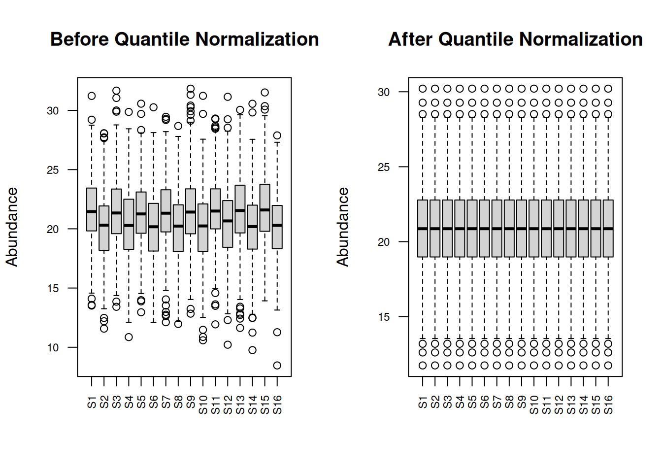

3.2.4.3 3. VSN (Variance Stabilizing Normalization)

# VSN normalization
vsn_fit <- vsn::vsn2(protein_matrix_imputed)
protein_matrix_vsn <- vsn::predict(vsn_fit, protein_matrix_imputed)

# Visualize mean-sd relationship
par(mfrow = c(1, 2))
vsn::meanSdPlot(protein_matrix_imputed, main = "Before VSN")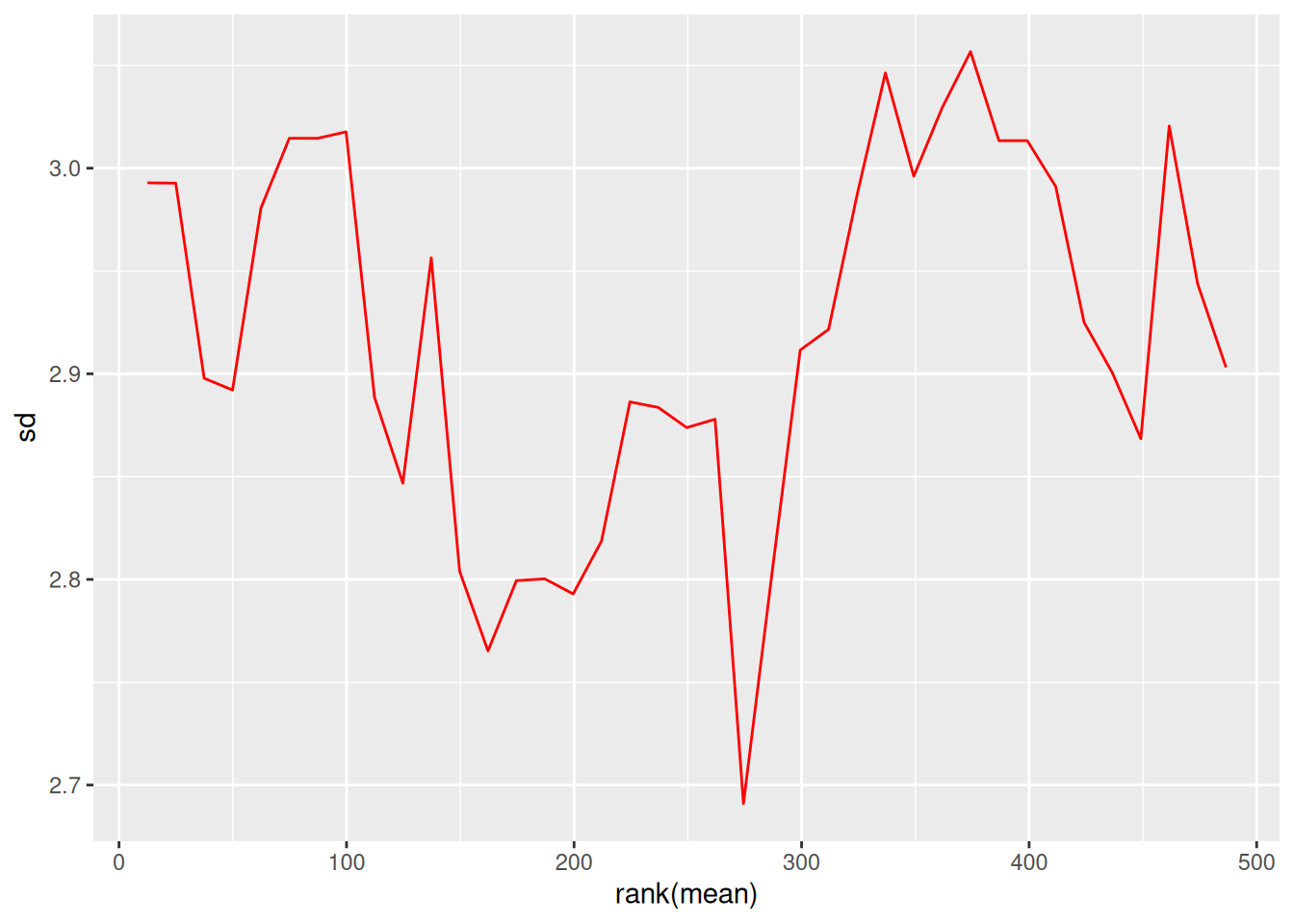

vsn::meanSdPlot(protein_matrix_vsn, main = "After VSN")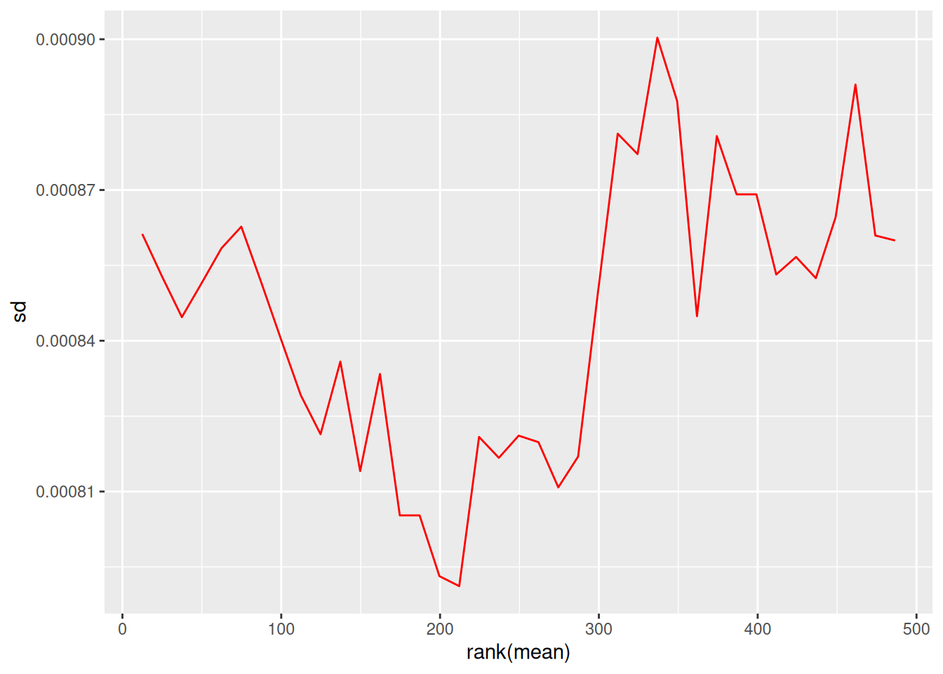

3.2.5 Comparing Normalization Methods

# PCA comparison
plot_pca <- function(data, title, metadata) {
  pca_result <- prcomp(t(data), scale. = FALSE)
  var_exp <- summary(pca_result)$importance[2, 1:2] * 100
  
  pca_df <- data.frame(
    PC1 = pca_result$x[, 1],
    PC2 = pca_result$x[, 2],
    condition = metadata$condition,
    batch = metadata$batch
  )
  
  ggplot(pca_df, aes(x = PC1, y = PC2, color = condition, shape = batch)) +
    geom_point(size = 3) +
    theme_minimal() +
    labs(title = title,
         x = paste0("PC1 (", round(var_exp[1], 1), "%)"),
         y = paste0("PC2 (", round(var_exp[2], 1), "%)")) +
    scale_color_brewer(palette = "Set1")
}

# Compare all methods
p1 <- plot_pca(protein_matrix_imputed, "Raw Data", sample_metadata)
p2 <- plot_pca(protein_matrix_median, "Median Normalized", sample_metadata)
p3 <- plot_pca(protein_matrix_quantile, "Quantile Normalized", sample_metadata)
p4 <- plot_pca(protein_matrix_vsn, "VSN Normalized", sample_metadata)

library(gridExtra)
grid.arrange(p1, p2, p3, p4, ncol = 2)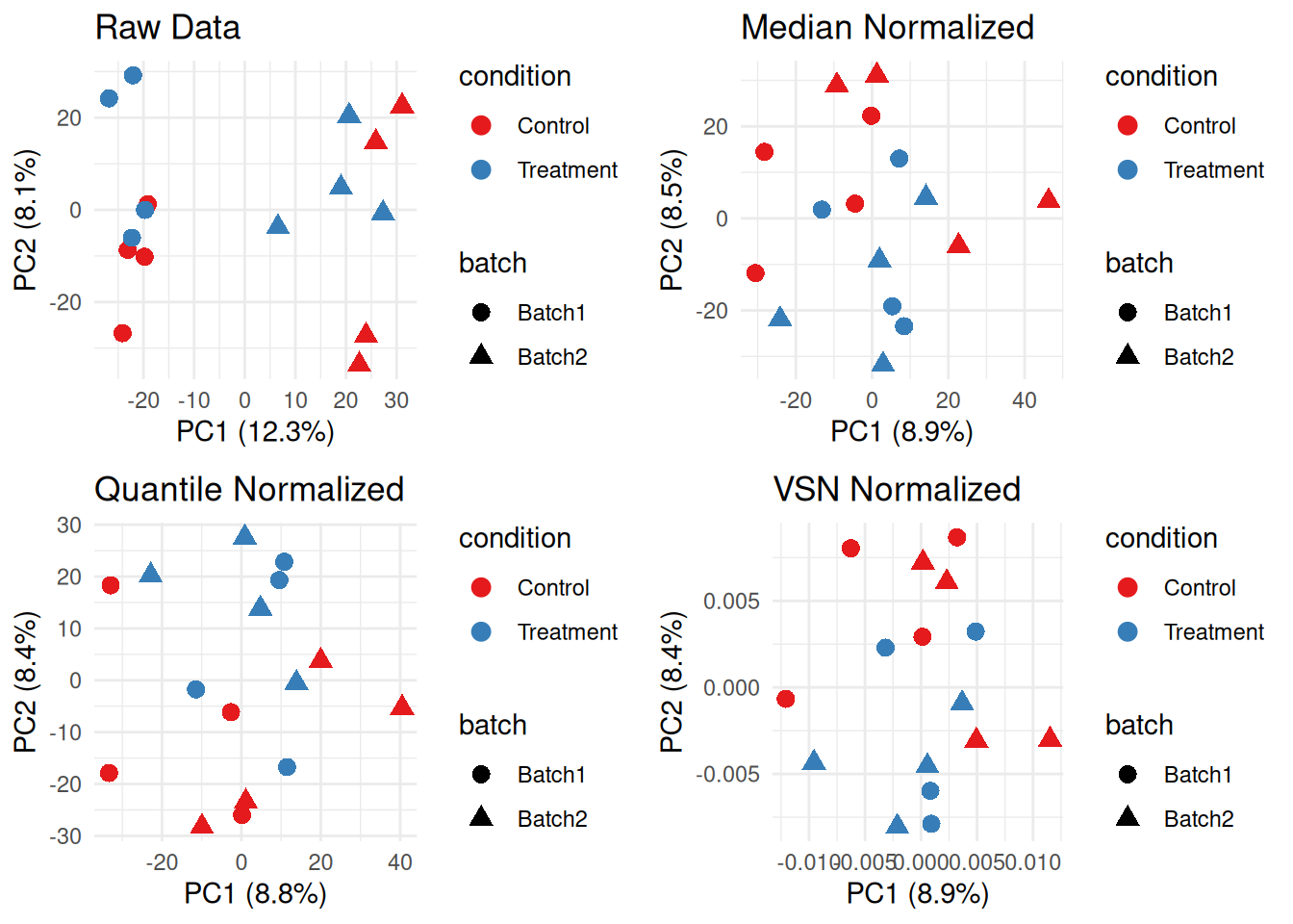

3.2.6 Exercise 3.1: Apply Normalization

Apply all three normalization methods and:

Calculate CV for each method
Compare sample correlations
Choose the best method for your data

# Solution
calculate_mean_cv <- function(data) {
  cvs <- apply(data, 1, function(x) sd(x, na.rm = TRUE) / mean(x, na.rm = TRUE) * 100)
  mean(cvs, na.rm = TRUE)
}

cat("Mean CV - Raw:", round(calculate_mean_cv(protein_matrix_imputed), 2), "%\n")
#> Mean CV - Raw: 14.1 %
cat("Mean CV - Median:", round(calculate_mean_cv(protein_matrix_median), 2), "%\n")
#> Mean CV - Median: 13.64 %
cat("Mean CV - Quantile:", round(calculate_mean_cv(protein_matrix_quantile), 2), "%\n")
#> Mean CV - Quantile: 13.67 %
cat("Mean CV - VSN:", round(calculate_mean_cv(protein_matrix_vsn), 2), "%\n")
#> Mean CV - VSN: 0.01 %

# Sample correlations
cor_raw <- mean(cor(protein_matrix_imputed)[upper.tri(cor(protein_matrix_imputed))])
cor_median <- mean(cor(protein_matrix_median)[upper.tri(cor(protein_matrix_median))])
cor_quantile <- mean(cor(protein_matrix_quantile)[upper.tri(cor(protein_matrix_quantile))])

cat("\nMean sample correlation - Raw:", round(cor_raw, 3), "\n")
#> 
#> Mean sample correlation - Raw: 0.024
cat("Mean sample correlation - Median:", round(cor_median, 3), "\n")
#> Mean sample correlation - Median: 0.024
cat("Mean sample correlation - Quantile:", round(cor_quantile, 3), "\n")
#> Mean sample correlation - Quantile: 0.024

3.3 Module 2: Batch Effect Correction

3.3.1 Detecting Batch Effects

# PCA colored by batch
pca_result <- prcomp(t(protein_matrix_quantile), scale. = TRUE)
var_exp <- summary(pca_result)$importance[2, 1:2] * 100

pca_df <- data.frame(
  PC1 = pca_result$x[, 1],
  PC2 = pca_result$x[, 2],
  sample_id = colnames(protein_matrix_quantile)
)
pca_df <- merge(pca_df, sample_metadata, by = "sample_id")

# Plot by batch
p_batch <- ggplot(pca_df, aes(x = PC1, y = PC2, color = batch, shape = condition)) +
  geom_point(size = 4) +
  theme_minimal() +
  labs(title = "PCA - Batch Effect Visible",
       x = paste0("PC1 (", round(var_exp[1], 1), "%)"),
       y = paste0("PC2 (", round(var_exp[2], 1), "%)")) +
  scale_color_manual(values = c("Batch1" = "red", "Batch2" = "blue"))

print(p_batch)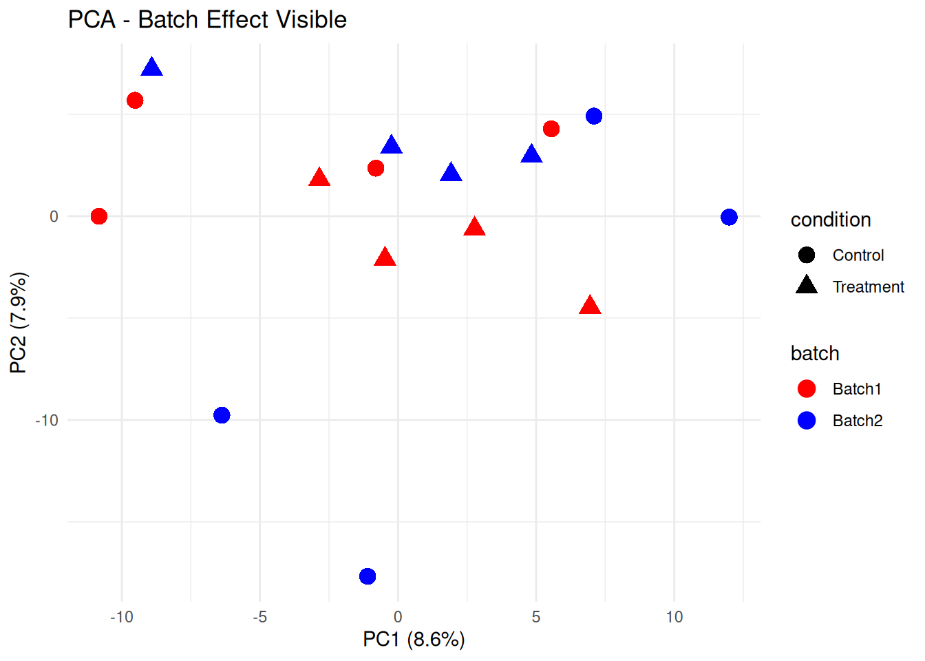

3.3.2 ComBat Batch Correction

# Prepare for ComBat
batch_vector <- sample_metadata$batch
condition_matrix <- model.matrix(~condition, data = sample_metadata)

# Apply ComBat
protein_matrix_combat <- sva::ComBat(
  dat = protein_matrix_quantile,
  batch = batch_vector,
  mod = condition_matrix,
  par.prior = TRUE,
  prior.plots = FALSE
)

# Compare before and after
pca_combat <- prcomp(t(protein_matrix_combat), scale. = TRUE)
var_exp_combat <- summary(pca_combat)$importance[2, 1:2] * 100

pca_df_combat <- data.frame(
  PC1 = pca_combat$x[, 1],
  PC2 = pca_combat$x[, 2],
  sample_id = colnames(protein_matrix_combat)
)
pca_df_combat <- merge(pca_df_combat, sample_metadata, by = "sample_id")

p_combat <- ggplot(pca_df_combat, aes(x = PC1, y = PC2, color = batch, shape = condition)) +
  geom_point(size = 4) +
  theme_minimal() +
  labs(title = "PCA - After ComBat Correction",
       x = paste0("PC1 (", round(var_exp_combat[1], 1), "%)"),
       y = paste0("PC2 (", round(var_exp_combat[2], 1), "%)")) +
  scale_color_manual(values = c("Batch1" = "red", "Batch2" = "blue"))

library(gridExtra)
grid.arrange(p_batch, p_combat, ncol = 2)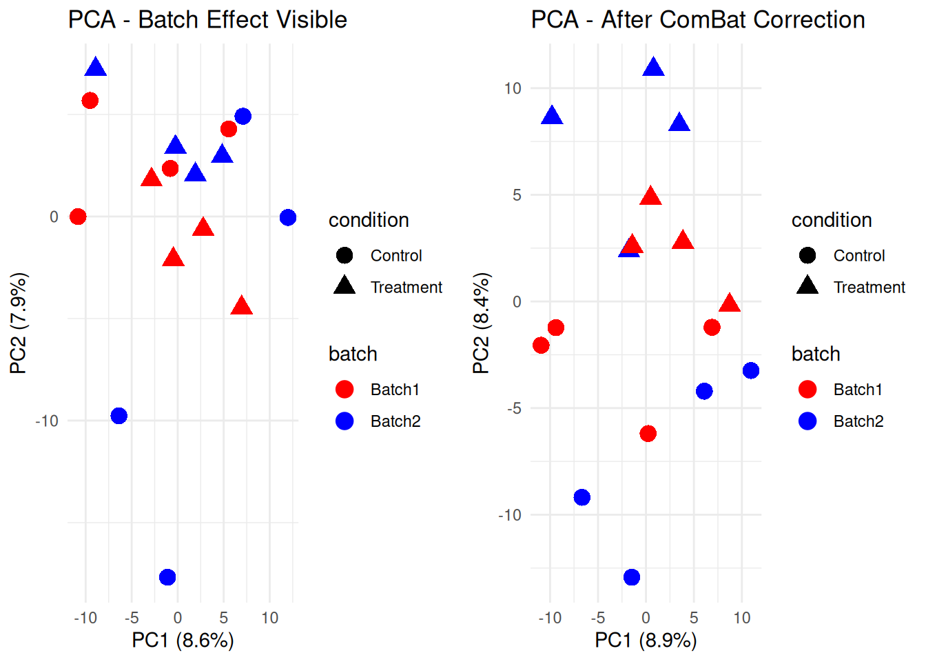

3.3.3 Scaling Methods

# Z-score scaling (by protein)
protein_matrix_scaled <- t(scale(t(protein_matrix_combat)))

# Pareto scaling
protein_matrix_pareto <- t(scale(t(protein_matrix_combat))) / sqrt(apply(protein_matrix_combat, 1, sd, na.rm = TRUE))

rownames(sample_metadata) <- sample_metadata$sample_id

# Visualize effect of scaling
pheatmap(protein_matrix_combat[1:50, ],
         scale = "row",
         main = "Heatmap with Row Scaling",
         show_rownames = FALSE,
         annotation_col = sample_metadata[, c("condition", "batch"), drop = FALSE])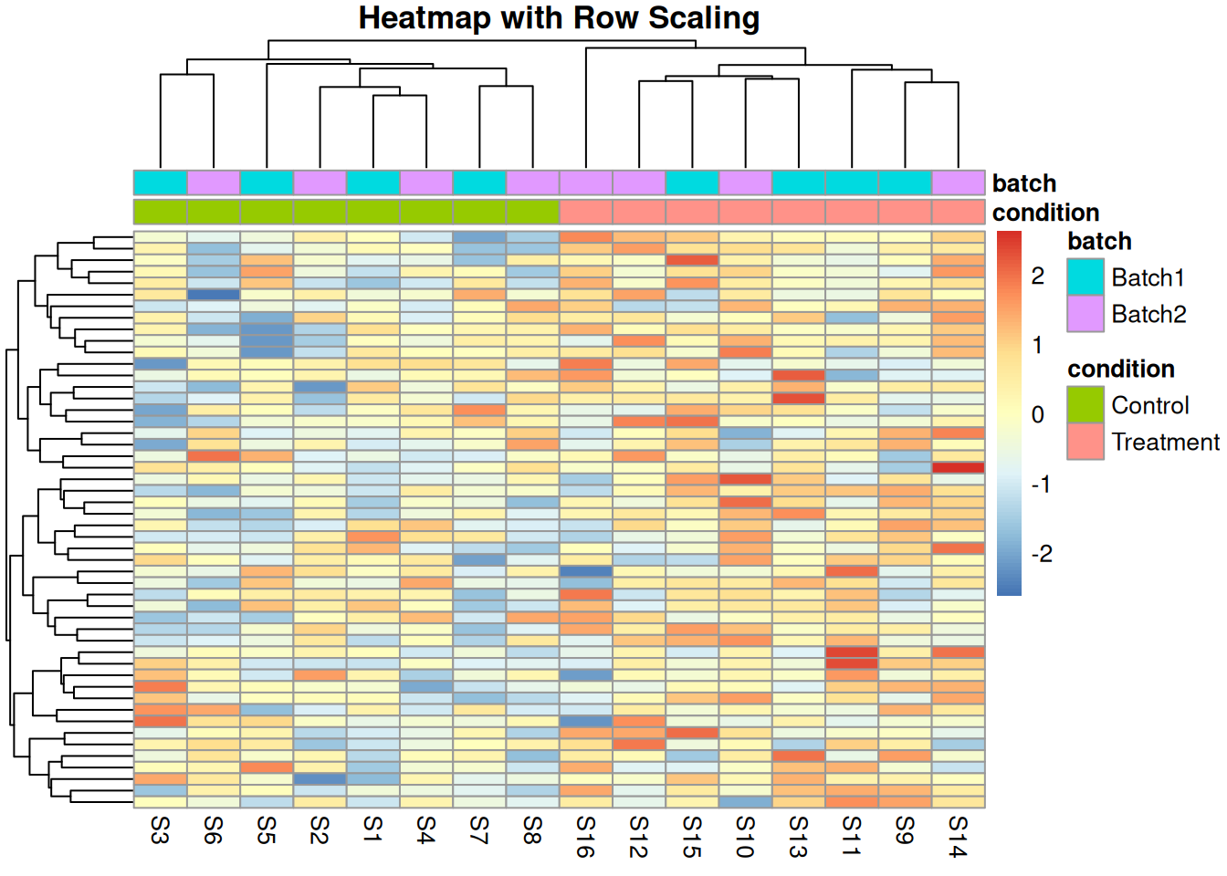

3.3.4 Exercise 3.2: Complete Preprocessing Pipeline

Create a complete preprocessing function that:

Filters proteins with >30% missing
Imputes missing values
Applies normalization
Corrects for batch effects

# Solution
preprocess_proteomics <- function(raw_data, metadata, 
                                   missing_threshold = 0.3,
                                   norm_method = "quantile") {
  # Step 1: Filter
  missing_per_protein <- rowSums(is.na(raw_data)) / ncol(raw_data)
  filtered_data <- raw_data[missing_per_protein <= missing_threshold, ]
  cat("Filtered to", nrow(filtered_data), "proteins\n")
  
  # Step 2: Impute
  imputed_data <- filtered_data
  for (i in 1:nrow(imputed_data)) {
    missing_idx <- is.na(imputed_data[i, ])
    if (any(missing_idx)) {
      imputed_data[i, missing_idx] <- mean(imputed_data[i, ], na.rm = TRUE)
    }
  }
  cat("Imputed", sum(is.na(filtered_data)), "missing values\n")
  
  # Step 3: Normalize
  if (norm_method == "quantile") {
    normalized_data <- limma::normalizeBetweenArrays(imputed_data, method = "quantile")
  } else if (norm_method == "median") {
    sample_medians <- apply(imputed_data, 2, median)
    global_median <- median(sample_medians)
    normalized_data <- sweep(imputed_data, 2, sample_medians - global_median)
  }
  cat("Applied", norm_method, "normalization\n")
  
  # Step 4: Batch correction
  if ("batch" %in% colnames(metadata)) {
    condition_matrix <- model.matrix(~condition, data = metadata)
    corrected_data <- sva::ComBat(
      dat = normalized_data,
      batch = metadata$batch,
      mod = condition_matrix,
      par.prior = TRUE,
      prior.plots = FALSE
    )
    cat("Applied ComBat batch correction\n")
  } else {
    corrected_data <- normalized_data
  }
  
  return(corrected_data)
}

# Apply pipeline
processed_data <- preprocess_proteomics(protein_matrix_raw, sample_metadata)
#> Filtered to 499 proteins
#> Imputed 495 missing values
#> Applied quantile normalization
#> Applied ComBat batch correction

3.4 Module 3: Differential Expression Analysis

3.4.1 Introduction to limma

limma (Linear Models for Microarray Data) is widely used for differential expression.

Key advantages: - Empirical Bayes moderation - Handles complex designs - Works well with small sample sizes

3.4.2 Basic Differential Expression

# Design matrix
design <- model.matrix(~0 + condition, data = sample_metadata)
colnames(design) <- c("Control", "Treatment")

# Fit linear model
fit <- lmFit(processed_data, design)

# Define contrast
contrast_matrix <- makeContrasts(
  TreatmentVsControl = Treatment - Control,
  levels = design
)

# Fit contrasts
fit2 <- contrasts.fit(fit, contrast_matrix)

# Empirical Bayes moderation
fit2 <- eBayes(fit2)

# Extract results
results <- topTable(fit2, coef = "TreatmentVsControl", number = Inf)

# Add protein IDs
results$protein_id <- rownames(results)

# View top results
head(results, 10)
#>            logFC  AveExpr         t      P.Value  adj.P.Val
#> P00043  5.029106 21.80541  3.895339 0.0001918769 0.06177827
#> P00026  5.054234 21.53741  3.730775 0.0003393640 0.06177827
#> P00439  5.116733 19.94913  3.704324 0.0003714124 0.06177827
#> P00041  4.754682 21.88690  3.521085 0.0006863510 0.07551792
#> P00050  4.458502 20.12443  3.472990 0.0008037582 0.07551792
#> P00448 -4.602952 20.09167 -3.435547 0.0009080311 0.07551792
#> P00204 -4.367604 20.06731 -3.373940 0.0011077982 0.07897018
#> P00037  4.021590 22.72349  3.151759 0.0022255595 0.13881927
#> P00326 -4.055987 20.17611 -3.083566 0.0027397386 0.15190329
#> P00025  3.882010 20.47140  2.992742 0.0035966903 0.17947484
#>                  B protein_id
#> P00043  0.51632573     P00043
#> P00026  0.04550759     P00026
#> P00439 -0.02887366     P00439
#> P00041 -0.53393668     P00041
#> P00050 -0.66346841     P00050
#> P00448 -0.76341971     P00448
#> P00204 -0.92614479     P00204
#> P00037 -1.49463286     P00037
#> P00326 -1.66317428     P00326
#> P00025 -1.88317691     P00025

# Summary
cat("\nDifferential Expression Summary:\n")
#> 
#> Differential Expression Summary:
cat("Significant proteins (FDR < 0.05):", sum(results$adj.P.Val < 0.05), "\n")
#> Significant proteins (FDR < 0.05): 0
cat("Upregulated (FC > 1.5, FDR < 0.05):", 
    sum(results$adj.P.Val < 0.05 & results$logFC > log2(1.5)), "\n")
#> Upregulated (FC > 1.5, FDR < 0.05): 0
cat("Downregulated (FC < -1.5, FDR < 0.05):", 
    sum(results$adj.P.Val < 0.05 & results$logFC < -log2(1.5)), "\n")
#> Downregulated (FC < -1.5, FDR < 0.05): 0

3.4.3 Volcano Plot

# Prepare data for volcano plot
volcano_data <- results
volcano_data$significance <- "NS"
volcano_data$significance[volcano_data$adj.P.Val < 0.05 & volcano_data$logFC > log2(1.5)] <- "Up"
volcano_data$significance[volcano_data$adj.P.Val < 0.05 & volcano_data$logFC < -log2(1.5)] <- "Down"

# Volcano plot
ggplot(volcano_data, aes(x = logFC, y = -log10(adj.P.Val), color = significance)) +
  geom_point(alpha = 0.6, size = 2) +
  scale_color_manual(values = c("Up" = "red", "Down" = "blue", "NS" = "grey")) +
  geom_hline(yintercept = -log10(0.05), linetype = "dashed") +
  geom_vline(xintercept = c(-log2(1.5), log2(1.5)), linetype = "dashed") +
  theme_minimal() +
  labs(title = "Volcano Plot: Treatment vs Control",
       x = "log2 Fold Change",
       y = "-log10 Adjusted P-value") +
  theme(legend.title = element_blank())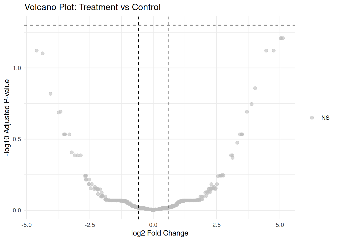

3.4.4 MA Plot

# MA plot
volcano_data$AveExpr <- results$AveExpr

ggplot(volcano_data, aes(x = AveExpr, y = logFC, color = significance)) +
  geom_point(alpha = 0.6, size = 2) +
  scale_color_manual(values = c("Up" = "red", "Down" = "blue", "NS" = "grey")) +
  geom_hline(yintercept = 0, linetype = "solid") +
  geom_hline(yintercept = c(-log2(1.5), log2(1.5)), linetype = "dashed") +
  theme_minimal() +
  labs(title = "MA Plot: Treatment vs Control",
       x = "Average Expression",
       y = "log2 Fold Change") +
  theme(legend.title = element_blank())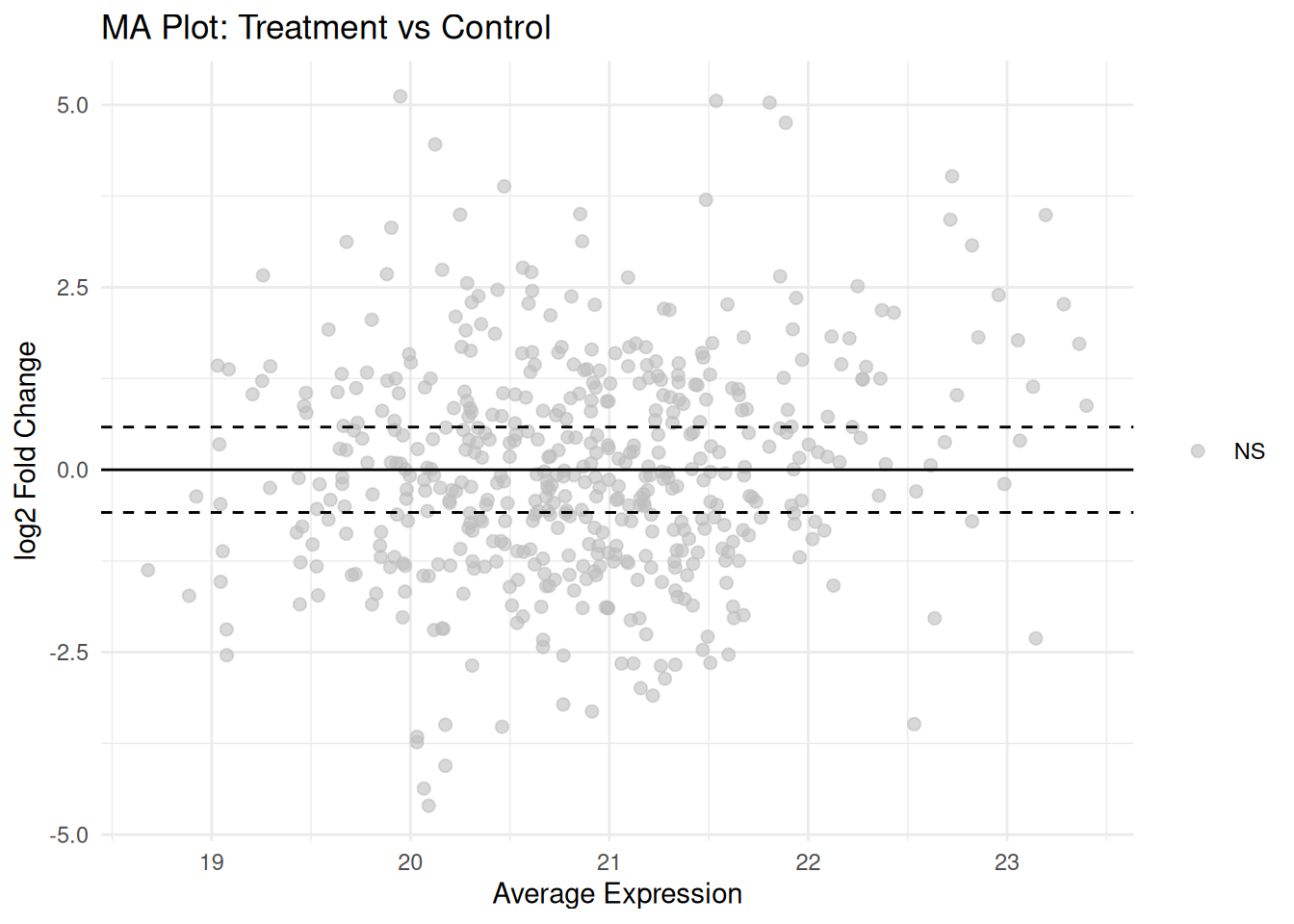

3.4.5 Heatmap of DE Proteins

# Select significant proteins
sig_proteins <- rownames(results[results$adj.P.Val < 0.05, ])

# Plot heatmap if there are significant proteins
if (length(sig_proteins) > 1) {
  pheatmap(processed_data[sig_proteins, ],
           scale = "row",
           clustering_distance_rows = "correlation",
           clustering_distance_cols = "euclidean",
           annotation_col = sample_metadata[, c("condition")],
           show_rownames = FALSE,
           show_colnames = TRUE,
           fontsize_col = 10,
           main = "Heatmap of Significantly Differentially Expressed Proteins")
} else {
  cat("Not enough significant proteins to generate a heatmap.\n")
}
#> Not enough significant proteins to generate a heatmap.

2 Introduction to Proteomic Data & Quality Control

4 Functional Analysis, Longitudinal & Public Data